Nervous network acceleration: quantitative measurement force

Quantity is a strong technique that is widely used in machine learning to reduce memory emissions and arithmetic requirements for nerve networks by converting floating separator numbers into correct low accuracy. This approach helps models to operate efficiently on compact devices and edge devices.

In this article, we will explore the quantitative selection in detail, carry out a small amount process, get rid of scratch, and show how to use them inside Pytorch models.

What is quantum measurement?

Estimating nerve networks is the process of converting weights and activating the nerve network from high -resolution formats (usually 32 -bit floating point numbers, or floating 32) to low accuracy formats (such as 8 -bit proper numbers, or int8).

The main idea behind the quantitative measurement is the “pressure” of potential values ​​in order to reduce data volume and accelerate accounts.

Nervous networks have become larger and more complicated, but their applications are increasingly required to operate resource -restricting devices such as smartphones, wearable devices, controlled machines and edge devices. The quantitative measurement:

• Reducing the size of the form: For example, switching from Float32 to INT8 can reduce the model up to 4 times.
• Faster conclusion: The correct account is faster and more efficient in energy.
• Decreased memory requirements and domain width: This is very important for edge/IOT devices and guaranteed scenarios.

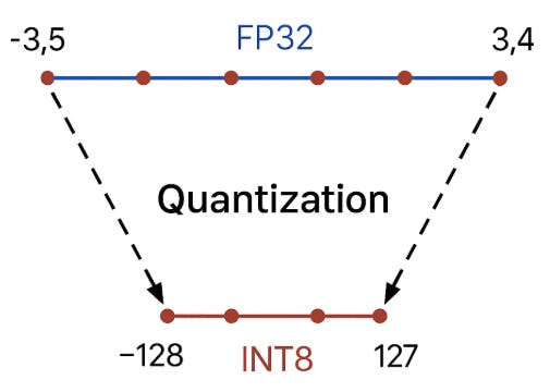
During quantitative measurement, weights and activation values ​​are set from the original ongoing range to separate levels using simple linear transformations.

For example, the scope of values [-3.5, 3.4] Slices can be to 256 level (INT8), and each real value is rounded to the nearest separate level.

In nerve networks, the most common measurement indicates the conversion of two types of data: weights and activation.

• Weights are the parameters that the network is “remembered” during training. They determine the strength of each input that affects the output of the neurons. The amount of weights can significantly reduce the size of the total model, because weights usually take most of the memory.

• Activation is calculated values ​​when taking out each layer while operating the network (inference). Basically, these are the “passed” signals from one layer to another. Activation is important to accelerate the inference because most of the operations within the nerve network are carried out on the activation.

The analog and similar measurement

When we make values ​​quantities, we need to “press” the original scope of the numbers and draw a map properly between Float and INT.

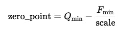
This is achieved using two main teacher size A laboratory indicates the amount of one step in representing a correct number that corresponds to the change in the value of the floating, and Zero_point – The value of a correct number determines the INT8 value that corresponds to zero in the representation of the float.

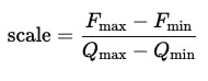
where
Fmax, Fmin– The maximum floor values ​​and minimum
Qmax, Qmin – The maximum and minimum values ​​of the correct number (127 and -128 for IN8)

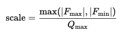
There are two main approaches: the analog and asymmetric measurement. The main difference between the analogous and similar measurement lies in how to set the original floating values ​​ranges into the correct quantitative numbers. With the similar measurement, the range of the floating value is always concentrated around zero (zero_point is 0), so zero in the field of flotation corresponds to zero in representing a correct number.

This simplifies the calculations and speeds up reasoning, but it requires almost the distribution of values ​​to both positive and negative sides.

On the contrary, the analogous measurement can work with any scope, not necessarily identical, and allows you to convert “zero” to the right point. This is achieved using a zero point, which determines the value of a correct number that corresponds to zero in the floating range. This approach is particularly appropriate when all values ​​in the tensioner are positive or contain a non -standard scale, for example, after applying the RLU activation.

In modern neurological networks, weights are often estimated in the same way, while activation is estimated as analogy, to achieve the best balance between accuracy and performance on real devices.

Formulas needed to supplement and get rid of: as follows:

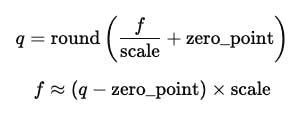
where

f The original floating value

q Quantitative value

Implementation of asymmetric quantum measurement in pytorch

This example explains how to perform the analogous measuring manually and get rid of the tensioner using Pytorch.

First, a random tensioner is created with Float32 values

import torch

# Generate a random 2D FP32 tensor (e.g., 4x5)
x_fp32 = torch.randn(4, 5) * 5
print("Original FP32 tensor:\n", x_fp32)

After that, the minimum and the maximum of this tension

# Find min/max for the whole tensor
x_min, x_max = x_fp32.min(), x_fp32.max()

qinfo = torch.iinfo(torch.int8)
qmin, qmax = qinfo.min, qinfo.max

# Calculate scale and zero_point for asymmetric quantization
scale = (x_max - x_min) / (qmax - qmin)
zero_point = int(torch.round(qmin - x_min / scale))

Next, the tensioner is converted into the correct number of INT8, values ​​are rounded, measured and converted to suit them in the correct InT8 range.

# Quantize to INT8
x_q = torch.clamp(torch.round(x_fp32 / scale + zero_point), qmin, qmax).to(torch.int8)
print("\nQuantized INT8 tensor:\n", x_q)

For test purposes, quantitative values ​​are again converted into the original FLOAT32 range using the reverse formula.

# Dequantize back to FP32
x_dequant = (x_q.float() - zero_point) * scale
print("\nDequantized FP32 tensor:\n", x_dequant)

Finally, quantum measuring errors -MEAN (MSE) and the maximum absolute error between the original and usual tensioner.

# Compare: MSE and max absolute error
mse = torch.mean((x_fp32 - x_dequant) ** 2)
max_abs_err = (x_fp32 - x_dequant).abs().max()
print(f"\nMSE between original and dequantized: {mse:.6f}")
print(f"Max absolute error: {max_abs_err:.6f}")

This example clearly shows how the main steps of the asymmetric quantities in practice work, and what types of abnormalities can occur when converting between floating representations and the correct number.

Below is the output of the code:

Original FP32 tensor:
 tensor([[ 2.8725,  1.0017, -4.8329, -0.8561,  2.7119],
        [ 9.3110, -2.9099, -9.1575,  7.8362,  4.5481],
        [-2.4224,  6.4360,  1.0812, -8.9195,  7.3958],
        [-1.5830, -1.7517,  4.6271, -9.3345, -9.3382]])

Quantized INT8 tensor:
 tensor([[  39,   14,  -66,  -12,   37],
        [ 127,  -40, -125,  107,   62],
        [ -33,   88,   15, -122,  101],
        [ -22,  -24,   63, -128, -128]], dtype=torch.int8)

Dequantized FP32 tensor:
 tensor([[ 2.8522,  1.0239, -4.8268, -0.8776,  2.7060],
        [ 9.2880, -2.9254, -9.1417,  7.8253,  4.5343],
        [-2.4134,  6.4358,  1.0970, -8.9223,  7.3865],
        [-1.6089, -1.7552,  4.6074, -9.3611, -9.3611]])

MSE between original and dequantized: 0.000275
Max absolute error: 0.026650

As you can see from calculated standards, the error between the quantum tensioner and the original tensioner is very small, and in most cases, it is hardly mentioned to the practical tasks.

After the similar quantitative training of the linear layer

In this section, we implement and test a simple linear layer with a similar amount after training.

thePTQSymmetricQuantizedLinear The separation extends nn.Module It mimics a standard layer completely connected, but adds the ability to determine its weights after training using the analogous measurement of 8 bits.

After training, we can call quantize_weights() The way the flos32 weights are used to the quantitative InT8 values ​​and store the corresponding scale. During reasoning (forwardThe layer rebuilds the original weights of its quantitative representation and calculates the output as usual.

import torch
import torch.nn as nn
import torch.nn.functional as F

class PTQSymmetricQuantizedLinear(nn.Module):
    def __init__(self, in_features, out_features, bias=True):
        super().__init__()
        self.in_features = in_features
        self.out_features = out_features

        self.weight = nn.Parameter(torch.empty(out_features, in_features))
        if bias:
            self.bias = nn.Parameter(torch.empty(out_features))
        else:
            self.register_parameter('bias', None)

        # buffers for storing quantized weights and scale
        self.register_buffer('weight_q', None)
        self.register_buffer('weight_scale', None)

    @staticmethod
    def symmetric_quantize(x):
        qmax = 127
        max_abs = x.abs().max()
        scale = max_abs / qmax if max_abs > 0 else 1.0
        x_q = torch.round(x / scale).clamp(-qmax, qmax)
        return x_q.to(torch.int8), torch.tensor(scale, dtype=torch.float32, device=x.device)

    def quantize_weights(self):
        w_q, w_scale = self.symmetric_quantize(self.weight.data)
        self.weight_q = w_q
        self.weight_scale = w_scale

    def forward(self, input):
        weight_deq = self.weight_q.float() * self.weight_scale
        return F.linear(input, weight_deq, self.bias)

Below, we explain how to create the layer, live weights, run inference, and compare the quantitative result with the original FLOAT32 output. This workflow clearly shows that identical measurement can pressure the model significantly while maintaining most of its numerical accuracy.

layer = PTQSymmetricQuantizedLinear(in_features=4, out_features=3)

# Initialize weights and bias for reproducibility
torch.manual_seed(0)
nn.init.uniform_(layer.weight, -1, 1)
nn.init.uniform_(layer.bias, -0.1, 0.1)

# Generate dummy input
x = torch.randn(2, 4)  # batch_size=2, in_features=4

# Quantize weights
layer.quantize_weights()

# Run forward pass
out = layer(x)
print("Output after quantization:", out)

# Compute the float32 (original) layer output
with torch.no_grad():
    out_fp = F.linear(x, layer.weight, layer.bias)
print("Output original float32:", out_fp)

# Compute the difference (MSE)
mse = torch.mean((out - out_fp) ** 2)
print("MSE between quantized and float32:", mse.item())

Below is the output of the code:

Output after quantization: tensor([[-0.2760,  0.6149, -0.0378],
        [-1.6489,  1.8015, -0.4852]], grad_fn=)
Output original float32: tensor([[-0.2753,  0.6172, -0.0395],
        [-1.6417,  1.8051, -0.4910]])
MSE between quantized and float32: 1.781566970748827e-05

conclusion

The main technology measurement that enables modern nerve networks not only on strong servers but also on resource -bound devices such as smartphones, wearable devices, mugs and edge devices. By converting weights and activations from FLOAT32 to the most compromise Int8 format, the models become much smaller, require less memory and calculation, and the inference times are significantly reduced.

In this article, we discovered how to make quantum measurement, discuss the differences between similar and asymmetric methods, and implement basic examples of these technologies in Pytorch, from manually identifying the tensioner to the post -training amount of nerve network layers.

Try it yourself on Jabbap

If you want to explore these practical examples, do not hesitate to visit my GitHub warehouse, as you will find all files for the symbol in this article. You can clone the warehouse, open the code in IDE or your favorite construction, and try it. Enjoy playing with examples!

Follow me

LinkedIn

Jaytab