Links table
Abstract and 1 introduction
1.1 Esprit and expand the central limit error
1.2 Contribution
1.3 Related work
1.4 Technical Overview and 1.5 Organizations
2 Evidence of measuring the central limit error
3 Evidence of the exhausting of the optimal error
4 second -class Eigenvertor theory
5 Strong EignVECTOR
5.1 Building “Good” p
5.2 Taylor expanded regarding the terms of error
5.3 Cancel the error in Taylor’s expansion
5.4 evidence of theory 5.1
Introductory
B Vandermonde Matrice
A deficient proof of Article 2
D proofs postponed for Article 4
The postponed proofs of Article 5
F lown Lond for spectral appreciation
Reference
The postponed proofs of Article 5
E.1 Evidence of Step 1: Building “Good” p


Who gives the expression of P eq. (5.2) in Lima.
II and II properties follow the claim E.2. Then the lemma guide is complete
E.1.1 Technical claims


guide. Note that


For the first chapter, we have


For the second period, we have


Combining them together, we have


Then the claim is continued.
The claim E.2 (the characteristics of “good” p). The reflective matrix P. specified by EQ. (5.2) satisfies the following characteristics:


guide. We fix each of the properties below.
Proof of property I:
By definition P (eq. (5.2)), our


Proof of property II:
It is considered


E.2 Evidence of Step 2: Taylor expanded regarding the terms of error
Lemma 5.3. Let p define it as eq. (5.2). Then, we have


According to the claim E.4, the Neumann series in EQ. (E.10) It can be taken until the second rank:


And for the remaining term, we have


Finally, combining EQS. (E.11) to (E.14) together, we get it


Where we reassemble the terms in the second step.
The lemma guide has been completed.
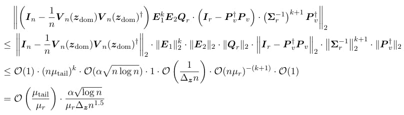
Lemma 5.4. It carries this


guide. We first deal with the term first demand in EQ. (5.8):


To the commitment (i), we notice


Combining this and reward. (5.4), we get it


Next, we keep (II) and look first in the term EQ. (5.8), which can be rewritten as follows:


Where the first two steps are followed by reinforcing terms, and the last step is followed by EQ. (E.22) and eq. (E.17).
Delivery of the border for the first order and the terms of the second order in EQ. (5.8) We get that


Who proves Lima.
E.2.1 Technical claims


It follows the first step of EQ. (1.13)


Follow the second step of inequality in a triangle, and the third step is followed by LEMMA 1.7 and Carollary B.2.
This means that


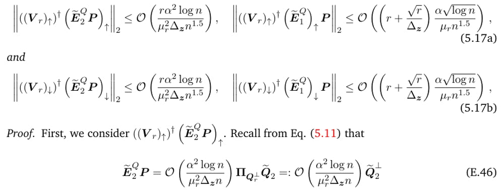
Claim E.4 (deduct the Neumann series). It carries this


guide. For the term Neumann series in EQ. (E.10):


We first link us to the middle arc:


The term first order (i.e., K = 1) in EQ. (E.21) It can be rounded as follows:


Where the first step follows the inequality in the triangle, follow the second step of EQ. (E.18) and eq. (E.22), and the last step is by direct account.
Through a similar account, we can make it clear that the second order (i.e., K = 2) in EQ. (E.21) can be rounded


In fact, this term can be simplified:


Where the first step follows the inequality in the triangle, follow the second step of EQ. (E.18) and eq. (E.22), and the last step is followed by the engineering summary.
Combining eq. (E.23) to eq. (E.26) Together, we get it


Then prove the claim.
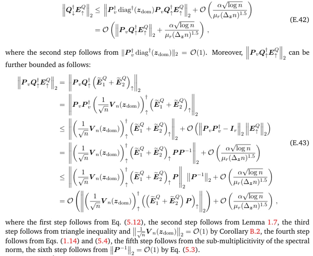
E.3 Evidence of Step 3: Cancel the error in Taylor’s expansion
E.3.1 Create the first equation in EQ. (5.10)


guide. In this guide, we often use the following notes:


It has been proven in the claim E.5.


Our

Where the third step LEMMA 1.7 is used for the first semester, EQ. (C.1) for the second chapter, Lemma C.1 for the third chapter, eq. (1.14) For the fifth and seventh chapters, equivalent. (B.2) for the sixth chapter. thus,


To link the second term in the above equation, for any K ≥ 0, we have


So, we get that


Likewise, we also have


Fire dam. (E.30) in EQ. (E.28) and eq. (E.29), Our


The lemma guide has been completed.
Lemma 5.6.


guide. We analyze eq. (5.13B) and eq. (5.13C) Pillar after another.


Combining the two equals above together and summarizing K, we get that


By eq. (5.13B) and eq. (5.13C), Our


Without a public loss, we only consider the first column of EQ. (E.33):


Where it follows the second step of the patience structure of the matrix. Therefore, by inequality in a triangle,


It follows the second step of EQ. (E.35) -Eq. (E.37).
Now, we consider the first term from F1. Know


It follows the second step of EQ. (E.39). The above equivalent indicates that


Delivery K = 0 in eq. (E.35) and eq. (E.36), we get any K> 0


This means that


Thus, we get that


Combining eq. (E.44) and eq. (E.45) together, fixed Lima.
Lemma 5.9.


Then, we adhere to eq. (E.50) and eq. (E.51) separately.
To reward. (E.50), We have


To reward. (E.51), we notice that


Thus, combining eq. (E.52) and eq. (E.53) together, we get it


Therefore, we complete the Lima guide.
E.3.3 Technical claims


Thus, LHS from eq. (E.55) can be expressed as follows:


By proving a little average from the natural result B.2, it is easy to show this


Along with LEMMA 1.7, we get it


Which proves the first part of the claim.
After that, we fixed. (E.55B).
When k = 0, equivalent. (E.55B) becomes


Which follows from Lemma 1.7.
When K ≥ 1, we have


Likewise, it can limit the second period:


The third term can limit it:


Thus, to prove equal. (E.55B), it is sufficient to commit


It follows the first step of LEMMA 1.7, and the second step is followed by EQ. (1.14). Combining the three equations above together, we get them


It follows the second step of using the B.3 natural result. This proves the case of K = 1 of EQ. (E.55B).
And finally, by urging eq. (E.56) to (E.59), we can prove this to I ≥ 2,


This concludes EQ’s guide. (E.55B).
Claim E.6.


Then follow the claim.
Authors:
(1) Chayan Ding, Department of Mathematics, University of California, Berkeley;
(2) Ethan n. Brace, Department of Computing and Sports Science, California Institute of Technology, Pasadina, California, USA;
(3) Lynn, Department of Mathematics, University of California, Berkeley, Department of Applied Mathematics and Accounts Research, Lawrence Berkeley National Institute, and the Institute of Challenge for quantitative account, University of California, Berkeley;
(4) Ruwaiza Chang, Simons Institute for Computing Theory.


 has started small – check out these four latokines less than $ 10 can rise to $ 100 or more")